INTRODUCTION
Dear Steel-IQ user!
This document will take you step-by-step through the installation of the model and the use of its graphical user interface.
Steel-IQ is a complex piece of modelling and there might be still some bugs here and there. If anything goes wrong during the installation process or use or you have ideas on how to develop the model further, feel free to send us feedback via our feedback form or directly via mail [email protected]. Alternatively, you can just modify the code on your own! It is shared under Apache 2.0 license and thus can be leveraged for any purpose, including commercial ones!
Despite operating out of a for-profit company, we firmly believe in open-source assets and their power to drive the discussion forward by providing a common point of reference and staging ground for further development. We are proud to contribute again to a growing portfolio of open sustainability models – we hope it will aid you in all your steel discussions.
Steel-IQ Team, Systemiq
PREREQUISITES
System Requirements
The model is large, complex, and may take a long time to run. Because of a number of computations (e.g. solving trade optimization for multiple commodities, calculating technology NPV for each year and each plant, etc.), the model is quite demanding on computer resources and runtime: in our experience, it may take up to 20–25 Gb of RAM and 10–60 minutes per year modelled (i.e., from 4–5 hours up to a full day for a 2025–2050 simulation run, depending on your machine). In our experience, performance on Macs with M1/M2/M3 CPUs is substantially faster than on Windows machines.
Because of that, you may wish to run it for 1 to 2 years only at first (e.g. 2025–2026) to check everything is set up ok. Then, if the results were generated correctly, you can go ahead and run a longer period. For larger simulations, you could process this overnight to minimize any performance issues during your working day.
Enter your details here to receive an email with download links to the Steel-IQ app and model:
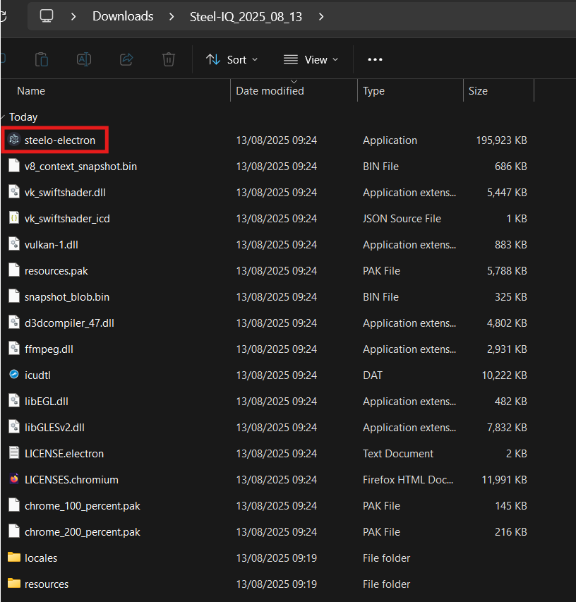
Right click the zip file and ‘Extract all’ files into your chosen folder (do NOT unpack it in “Program Files” or any system-adjacent folder, your OS may not like it!) Note please use a short path (in order not to trigger 260 characters maximum file path length limitation).
Open the folder where you extracted the zip file and double click on “Steel-IQ” application.
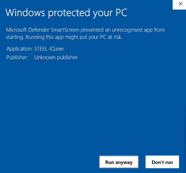
There might be a warning pop-up, click “Run anyway”
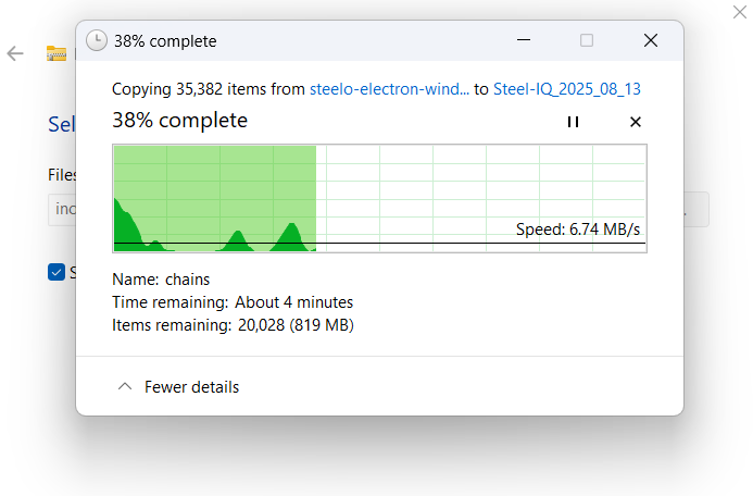
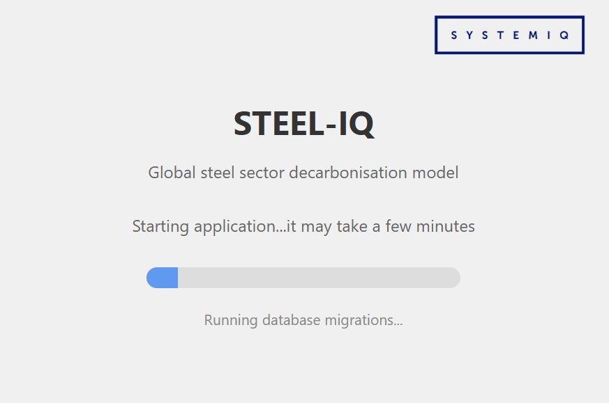
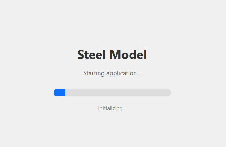
Steel-IQ will let you know that it is initializing with a progress bar. It may take few minutes…
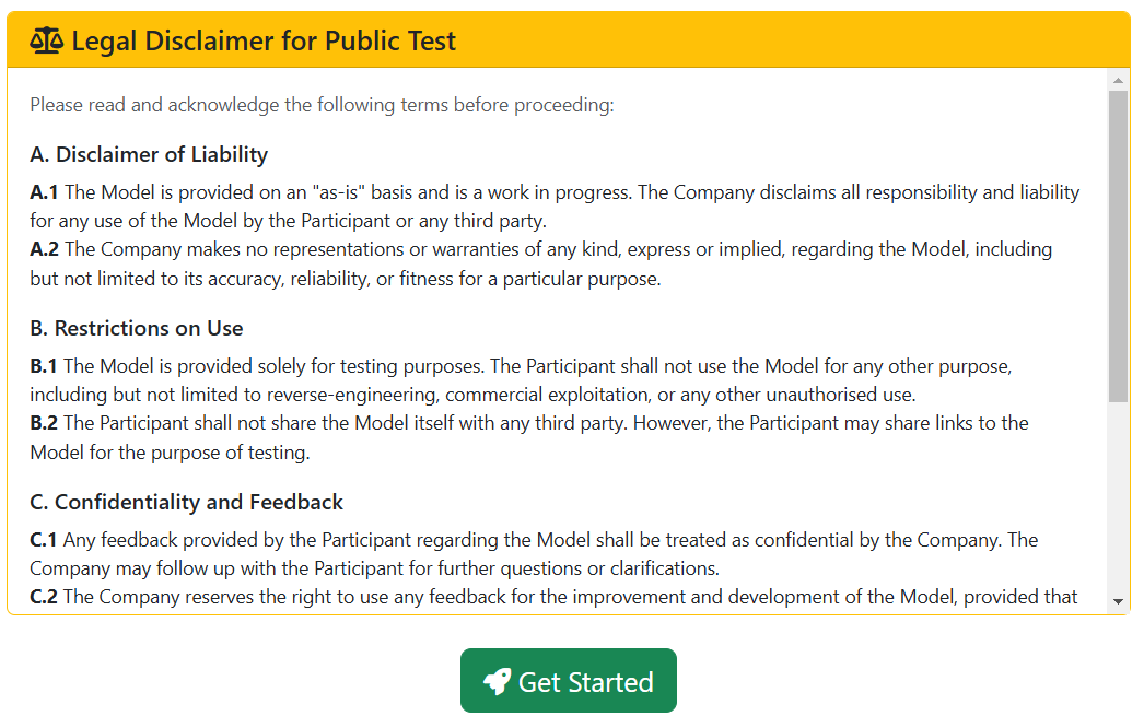
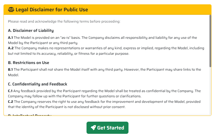
You have to accept a legal disclaimer to use the model. Do not worry, the license is very permissive as long as you quote us whenever you use/expand the model.
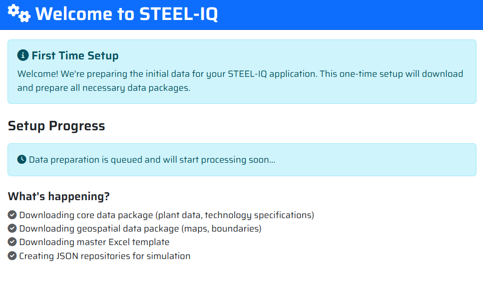
The app will set itself up in terms of required libraries/packages and data structures. This may take a little time as the file sizes are large.
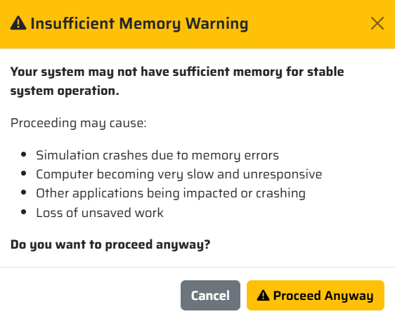
Amemory warning may appear. In our experience, model usually runs well with 16 Gb of RAM and more, but may run out of memory if you have less (and sometimes 16 Gb will be not enough).
Enter your details here to receive an email with download links to the Steel-IQ app and model:
1. Check your Mac
Apple menu → *About This Mac* → confirm the chip line says “Apple M1/M2/M3…”.
We only publish an ARM64 build; Intel Macs should use the hosted web version or the Windows package via virtualisation.
Ensure at least **16 GB of RAM** and 10 GB of free disk space for the initial data download.
2. Download the archive via Terminal
a. Press `⌘` + Space, type `Terminal`, press Return.
b. In the new window paste the command from the Steel-IQ download page, for example:
“`
cd ~/Downloads
curl -L <insert here the link to the file you receive in an e-mail> -O
“`
Why not just download through the browser? Using `curl` keeps the file free of the browser quarantine flag so Gatekeeper will not mark it as “damaged”.
3. Unpack the application
“`
tar xzvf <insert here the name of the file from the download link in the format: STEEL-IQ-macos-<date, time and build ID>.tar.gz>
“`
This creates a `mac-arm64` folder with `STEEL-IQ.app` inside.
4. Open the folder in Finder
“`
cd mac-arm64
open .
“`
Finder opens the folder so you can drag `STEEL-IQ.app` into `/Applications` (recommended) or another location you prefer.
5. Launch Steel-IQ
– Double-click `STEEL-IQ.app`. The first launch prepares datasets; expect a progress bar that can take 2–15 minutes depending on hardware. Leave the window open until the progress bar finishes.
6. If macOS reports the app as damaged
-This can happen if the file was downloaded with Safari/Chrome.
In Terminal:
“`
xattr -dr com.apple.quarantine /Applications/STEEL-IQ.app
“`
Then try launching again via Finder (Right-click → Open if macOS still prompts about the unidentified developer).
7. Troubleshooting
Still on Intel hardware? Reach out to the team for remote-access options—this build will not start on Intel Macs.
You have to accept a legal disclaimer to use the model. Do not worry, the license is very permissive as long as you quote us whenever you use/expand the model.
The app will set itself up in terms of required libraries/packages and data structures. This may take a little time as the file sizes are large.
A memory warning may appear. In our experience, model usually runs well with 16 Gb of RAM and more, but may run out of memory if you have less (and sometimes 16 Gb will be not enough).
MODELLING SCENARIOS
User Guide
To model the scenarios you have in mind, you can adjust the simulation parameters in 2 main ways:
A- Through the “New simulation” input dashboard. For the final model, this will be a go-to option, but currently relatively few simulation parameter controls are linked to the dashboard;
B- Through editing and uploading the “Master Excel file”. This is the most flexible way, as you are able to adjust a wide array of model inputs (e.g., trade tariffs, carbon costs or commodity prices in a specific year). To do that:
- Download the template,
- Edit the values to your liking while preserving the file and worksheet structure and units of measure,
- Upload the saved file into the model,
- Prepare the file (for model to be use it),
- Create and run a simulation, and download your results.
More detailed instructions are included in the “Master Excel file” in the worksheet “Instructions” (and below)…
GETTING STARTED
Once initialized you will have access to two main panels in the model: “Master Excel” and “Simulations”
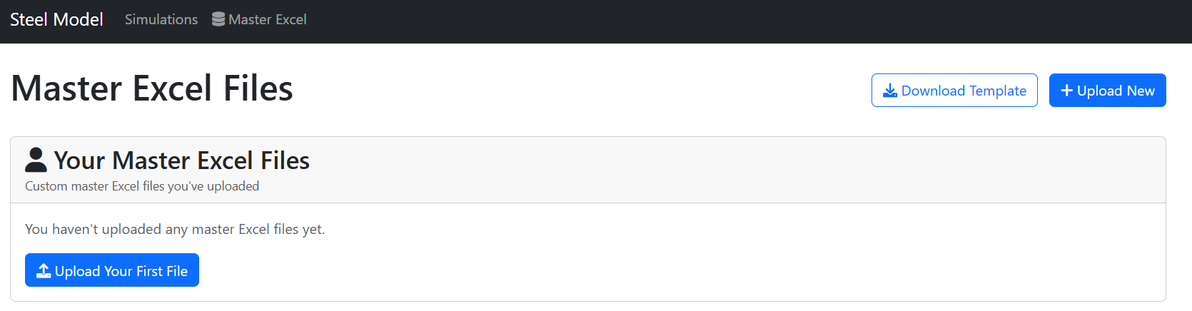
Master Excel
Here you will upload the excel input. We call it “Master Excel” because of its importance to the model run and how much data points it covers. We believe it is quite useful on its own. This panel is very simple, you can essentially do two things:
Download Template – downloads the Master Excel file. If you do not want to/need to customize all the inputs, fear not – default values are there for your convenience.
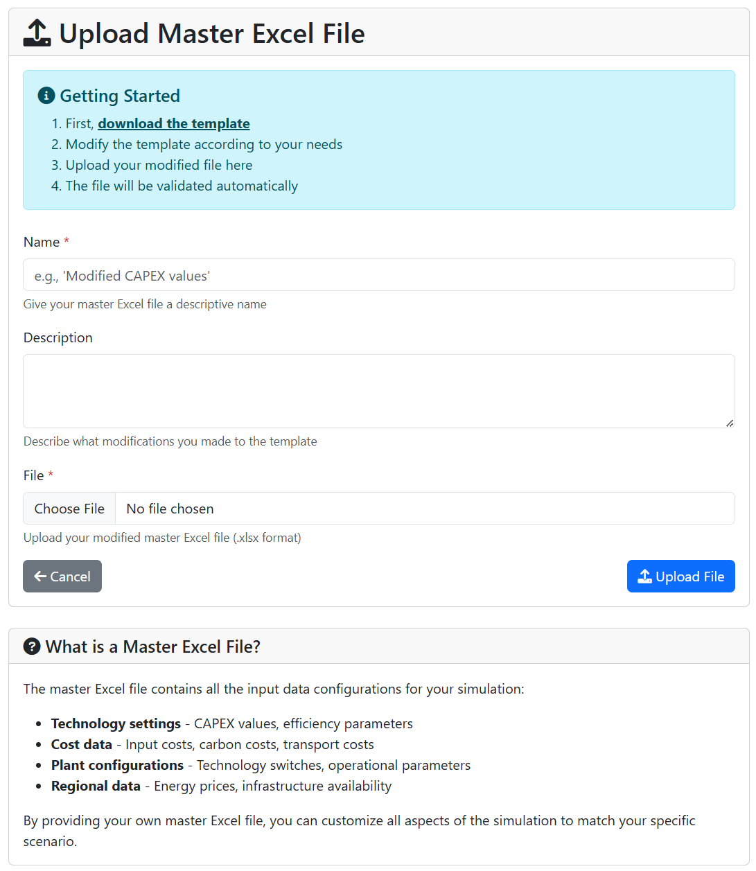
Upload File – opens up another panel where you can upload your customized Master Excel the following way:
- Give it a unique “Name” (please note it is possible to run multiple scenarios in one go, so making the name unique can go a long way),
- Provide a more detailed “Description” if needed,
- Browse your machine to get the right “File”,
- Once you are set, click “Upload File” and let the magic happen.
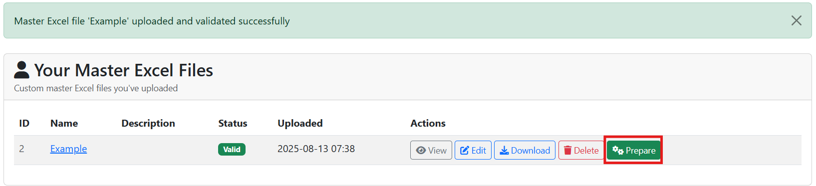
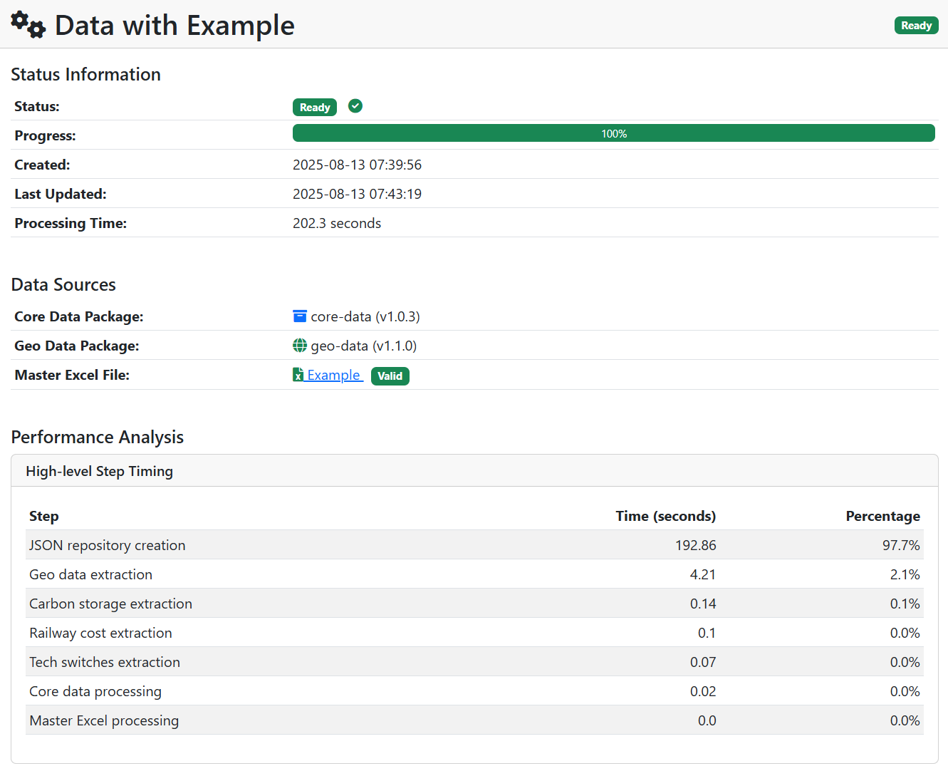
Once the Excel file is successfully uploaded to the model, click a green “Prepare” button so the input data is read in. This step also performs an integrity check to see whether there are no missing sheets. Word of warning, though: it does not check for the correct units or format of the inputs (we do our best to handle that inside the Master Excel). Make sure you follow the units in the file.
Note: We advise to run the model for 1-2 years, check whether results make sense, and only then commit to a longer peroid.
Once the data extraction finishes, it will show some statistics on how long it took. If it fails, it should flag at what stage it encountered an error to aid in troubleshooting.
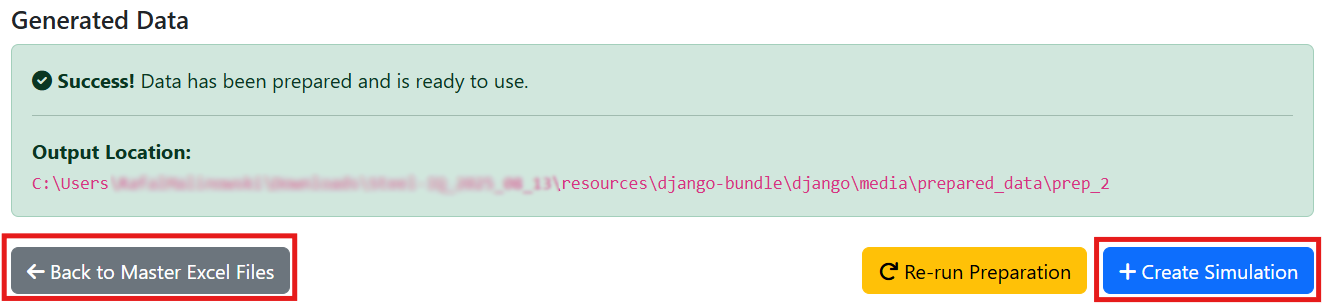
Once the Excel file is uploaded successfully, you are ready to go – you can either click “Create Simulation” to run an analysis with the newest input file you uploaded or go “Back to Master Excel Files” if you want to upload more of them (if you want to run multiple scenarios in one go)
Note: the demand and scrap availability projections come from our aptly named “Demand/Scrap Availability Model” which is a hefty model on its own. It has been made open-source as well and you can download it from the RESOURCES panel.
SIMULATIONS
- “Simulations” – here you can either “Browse Master Excel Files” and “Create Simulation”. At that stage there should be nothing surprising about the former, so let us cover the latter:
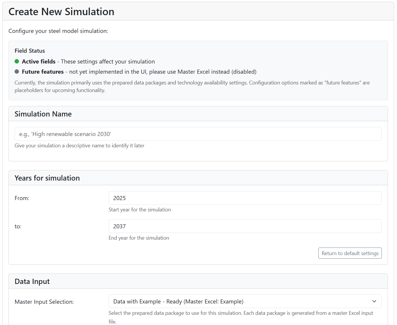
“Create Simulation” – here you are able to set up the next run of the model.
-
- “Simulation Name” – provide a unique name for the run
- “Years for simulation” – specify period for which you want to run the model
- “Data Input” – select the Maste Excel input file
- Once you are done with setting up the run, click “Create Simulation” at the bottom of the page
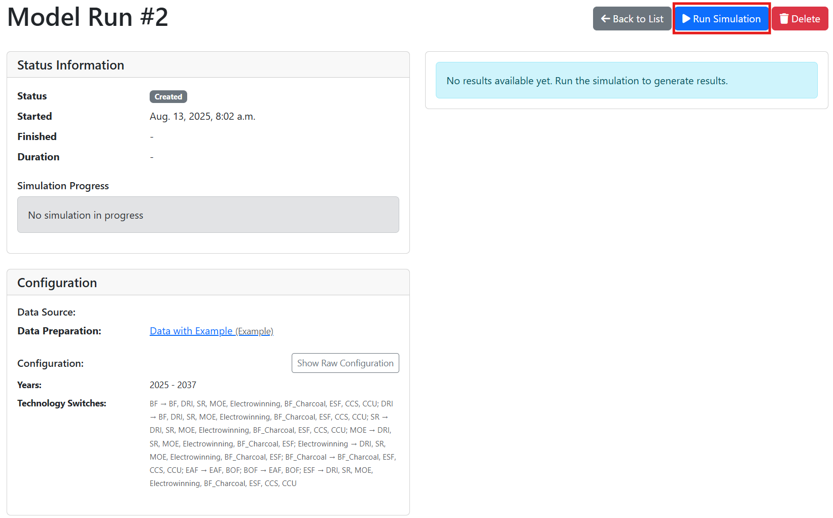
- The new panel will show you the progress of the simulation after you press “Run Simulation”
Performance & speed
- The model can take a lot of time to run. We did our best to prevent incorrect data to be loaded into the model, but there is a chance you will encounter an issue. The last thing you want to see is that the model you left to do its job for few hours failed after first year and aborted the whole run. Try running one year and only if this one works, go for the whole run.
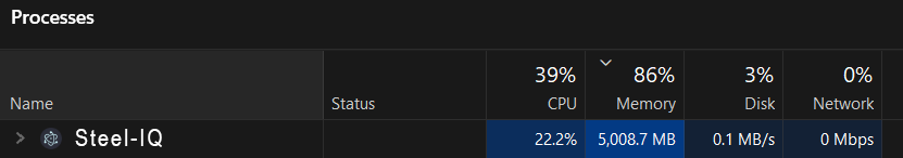
- As long as the “Status” says “Running”, it is fair to assume that everything is running correctly. If you are suspicious, you can also check in the Task Manager whether “Steel-IQ” grabbed its fair share of your machine’s memory.
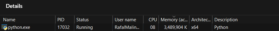
- What we also found useful is to go to more detailed breakdown of processes in the Task Manager and give python.exe higher priority for memory allocation (Right-click -> Set priority -> “High”) so it can claim more of the available RAM.
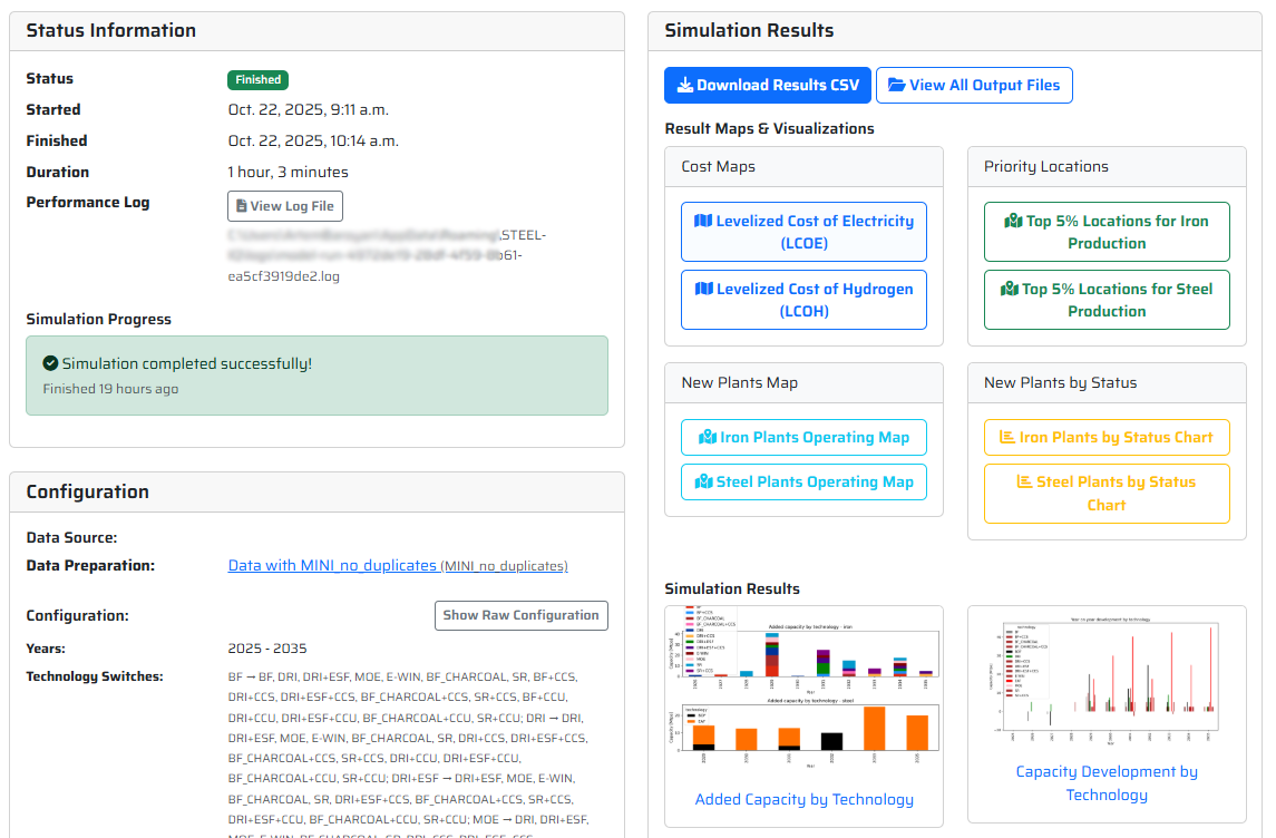
- “Download Results CSV” – allows you to download a comprehensive csv showing essentially all plant-level data (production, capacity, opex breakdown, the decisions made by each furnace group, etc.). The results might be a difficult to process at first glance, therefore we provided you with an Excel that should help you parse and understand them [link here]
- “View All Output Files” – here you can access more detailed results/charts, including trade results available both in .csv you can analyse and .html which are actually interactive trade maps you can easily review and share with others. At the top you can also see in which folder the data was stored in case you would like to move or process them in bulk.
Thats it- you should be able to use Steel-IQ to generate your own scenarios and results which can hopefully help you play your part in the push to decarbonise industrial steel production.
- If you have any further questions, please check out our extensive FAQ’s below, and if that does not help, reach out to us either via feedback form or mail us at [email protected]
FREQUENTLY ASKED QUESTIONS
FAQs
General understanding
The Steel-IQ model has been developed by Systemiq with philanthropic funding to inform discussion on steel decarbonisation. It is a global plant-level decarbonisation model where the user can test multiple technological, market and policy levers and how they might drive the iron and steel decarbonisation effort.
The model’s outcomes are meant to be used at global or regional level. Even though the model applies a plant-level perspective for granularity and nuance, it should not be understood as a credible tool for projecting the future of a single asset nor a digital twin of the industry for the following reasons:
- There is no detailed open-source asset-level financial and technological data that we are aware of,
- We did not capture the cost stack of each location perfectly. In order to do the analysis globally, we had to make certain high-level assumptions (i.e., fill in the blanks in country-level data with regional assumptions),
- We do not differentiate between finished steel products, which in real life is an important driver of steel plants’ economics,
- We do account for availability of logistical infrastructure, but the Open Street Maps we used for that purpose might be incomplete,
- We deployed simplified balance sheet modelling: we only account for the accrued profit/loss for the purpose of deciding whether the model decision-makers (e.g. plants) have enough equity for investments.
Steel-IQ explicitly models iron and steel plants, based on the Global Energy Monitor’s “Global Iron and Steel Tracker” which captures vast majority of the active capacity and is open to use. Because the dataset does not contain information about the age of each furnace in the plant, we bundle furnaces of one technology into a “furnace group” and treat them as units upon which decisions can be made. For the purpose of making the behaviour more realistic, we bundle the plants into corporate groups based on their Ultimate Parent Company.
When it comes to their suppliers, burden preparation steps (sintering, pelletising, coking) are assumed to be integrated within the ironmaking step. To optimize model run time, we had to make a decision on sinter vs pellet split for blast furnaces: we assumed 2:1 sinter to pellet ratio (in terms of their iron contribution).
Iron ore mines have set capacity and price/cost at which they provide the iron ore. The dataset is an aggregated S&P Capital IQ Pro iron ore database – we divided the iron ore grades into three large buckets depending the iron content and then aggregated those buckets per country with cost being a weighted average for a given country/region.
No financials nor decisions are modelled for the burden preparation and iron ore mining steps.
There are five main types of decisions that are made in the model:
- Continue operating (if the expected profits are good enough to continue producing),
- Close the asset (if accrued losses breach a certain threshold),
- Switch technology (if Net Present Value of switching to this technology is above 0 AND decision-maker has enough accrued profit to foot in the equity part of the investment),
- Expand capacity (in an existing location),
- Build new capacity (in a new location).
For each available option, the agent calculates an NPV (using country-/region-specific cost of capital and cash flows expected for a given asset), and generally selects the highest-NPV option. The simple highest-NPV logic was found to be too simplistic and a set of constraints have been introduced to make asset-level behaviour more realistic:
- The NPV of a beneficial decision needs to be positive few years in a row (by default 3 years – think: executives need time to make sure it’s a worthwhile investment)
- Even a highly beneficial decision is subject to a certain maximum probability to happen each year (by default 70% – think: risk appetite and “stickiness” of status quo),
- A project which has been already announced (i.e., final investment decision taken) has a small chance to be cancelled (by default 10% – projects do get cancelled in real life for a variety of reasons).
All above parameters can be set in the “Global variables” tab in the Master Excel input file. The default has been set selected by trial and error and in order to keep the assets sensitive to shocks but not too much, i.e., we expect assets to be able to weather few bad years before making a decision about closure, similarly with expansion.
- Stock and flow model is used to determine country-level demand for steel and scrap availability (which, if changed by the user, has to be copied into the Master Excel input file – see point 4.)
- Geospatial data is used to generate location-specific cost of baseload renewable supply (-> Levelized Cost of Electricity, LCOE) and cost of baseload hydrogen provision (-> Levelized Cost of Hydrogen, LCOH).
- Additional criteria are added to the LCOE/LCOH map in order to create a map of potentially attractive locations for new iron- and steel plants. Example criteria are: distance from logistical infrastructure and expected transportation cost of feedstock and products.
- User opens a graphical user interface (“an executable”), downloads a pre-filled Master Excel input file and customizes the inputs for a given scenario.
- Few selected inputs are specified via the input dashboard of the executable.
- User uploads a single or multiple input files, the model validates their integrity, and then starts the simulation(-s).
- Results of the run are available either via the executable or in the folder shown in the executable after the run is done.
We set up a linear programming (LP) model that minimizes the total cost at which the demand nodes (=buyers of the final product, in our case crude steel) meet their demand. The total cost accounts for both production cost, transportation, and trade policies (i.e., tariffs or import/export quotas). The model also optimises the feedstock composition of iron and steel plants, following the constraints on feedstock availability.
We chose the LP formulation of the trade problem due to its flexibility (we can easily add new constraints, assets, and products). The drawback is unfortunately scalability – the computational time increases fast with increase in modelled assets, feedstock options, and constrains. That led to us to limiting the available feedstock options (i.e., we assumed that DRI made out of high-grade DR pellets will never be used in the Electric Smelting Furnace even though it is technically possible) and refraining from modelling the trade of energy vectors (both fossil and non-fossil). Otherwise, the model runtime would become excessive and even now it is not the shortest. Nonetheless, it should be noted that the LP framework does allow to include all those options, the question is only about the practicality of using the model.
Model scope & capabilities
Steelmaking, ironmaking, scrap supply, and the iron ore mining. Iron ore agglomeration steps (sintering, pelletising) and coking are weaved into the ironmaking.
Ironmaking: Blast Furnace, Direct Reduced Iron, Direct Reduced Iron with Electric Smelting Furnace, Molten Ore Electrolysis, Electrowinning, Charcoal Minifurnace, Smelting Reduction
Steelmaking: Basic Oxygen Furnace, Electric Arc Furnace
Other (applicable to all technologies with direct CO2 emissions): Carbon Capture and Storage, Carbon Capture and Utilisation
Yes, direct and indirect emission factors are specified across multiple system boundaries supported. Power grid-related emissions are based on country-level data, with gradual decrease in accordance with countries’ net-zero targets. For new plants, majority of power used is renewable-based.
- Iron ore mines have limited capacity for each of the grades,
- Scrap availability is finite and specified at country level,
- CO2 storage availability (for CCS) is limited at country level,
- Annual biomass availability is limited per high-level region.
Yes. Demand is modelled at country level using the stock and flow approach with tweakable high-level levers.
Inputs & data requirements
There are many metrics affecting the model and they are provided via a so-called “Master Input Excel” file which can be down- and uploaded from/to the model executable. Input metrics are prefilled for convenience. Some metrics can be changed/specified via the graphical user interface.
We precalculated a set of scenarios to showcase the capabilities of the model – you can access them via the RESOURCES section.
Generally yes. The demand and scrap availability datasets start way in the past. However, all the other inputs have to be extended into the past and then the correct time period has to be selected in the model executable (where the user specifies the period over which a scenario is supposed to run).
Decision logic & NPV calculation
We calculate levered NPV by summing up expected discounted revenue (based on the historical experience of a given asset) over investment horizon and deducting the expected discounted costs, incl. impact of upcoming policies. Because the NPV is levered, the debt repayment and interest are modelled explicitly as cash outflows (with interest calculated using cost of debt for a given country), discounted using a cost of equity.
The model uses country-level cost of debt and cost of equity, with missing data points filled in using the 3rd quartile cost of debt/equity for a given region (based on available data).
There are three main ways the future costs and revenues are estimated:
Cost:
- Existing plants have hold memory of the last several years (user-specified, X by default) and assume their cost stack will look the same until end of relevant investment horizon. The benefit of that approach is that the capacity utilisation is more realistic because it is based on already known past behaviour. The same applies to revenue – existing plants hold a memory of prices and production volumes and assume their average over X years will carry on until the end of investment horizon,
- Business case for expansion of capacity is evaluated using similar logic, but with the impact of potential expansion on iron or steel prices (added capacity may shift cost curve to the right, causing a decrease of a “clearing” price – hence worsening the economics for existing capacities),
- Business case for greenfield plants is evaluated using a standardized business case for each technology but using local cost of inputs. The simplification here is that the capacity utilisation is assumed to be equal to the global average which may deviate from the actually experienced utilisation factors for a given country. In addition, since there is no memory, steel price for the whole investment horizon is assumed to be equal to the price experienced in the last year.
Yes – there is a set of global variables governing behaviour of the model (i.e., probability of expanding the capacity if the business case seems profitable) which can be accessed via “Global variables” tab in the Master Input Excel.
Technical implementation
- Bulk of the model, incl. plant-level economics and trade: Python
- Geospatial module: Python with simplified Atlite-based workflow, parallelised using Dask
- Demand/scrap availability: Excel, using Python for fitting the s-curves between past data and projected steel stock saturation levels
- Graphical UI: Electron
The model uses open-source HiGHS solver. It cannot be changed without a code intervention
That depends mainly on the number of options available to the trade (LP) module and the performance of the machine you run the model on. Based on our tests on various machines, the default model with default dataset needs 20–25 Gb of RAM and 10–60 minutes per year modelled (i.e., from 4–5 hours up to a full day for a 2025–2050 simulation run, depending on your machine). In our experience, performance on Macs with M1/M2/M3 CPUs is substantially faster than on Windows machines. For efficiency, you can queue several simulations (e.g. with different decarbonization levers or other settings) to run them overnight or over a weekend.
Running & customising the model
- Using the graphic interface, you can then download, modify and upload back the modified Master Input File, and then create a simulation using that file – in that case you can test different hypotheses and see how different levers impact the outcomes. See the guide above…Alternatively, you can create a simulation using a default Master Input File and “baked-in” scenarios and values.
Should run on any modern laptop (PC or Mac) but reasonable runtimes likely require at least 16 Gb and preferably 24-32 Gb RAM.
Vast majority of the parameters are changed via a Master Input Excel file which can be downloaded from and uploaded to the model executable. Several the parameters (e.g. time horizon) need to be changed in the dashboard of the executable file when creating a simulation.
Yes – the model by default works with a large database of iron and steel plants. They can be gathered into one “portfolio” with a joint (simplified) balance sheet via the “Ultimate Parent” column.
We break down each plant into groups of furnaces sharing the same technology and many decisions are applied to a furnace group rather than the whole plant, so it is perfectly fine if there are two ironmaking technologies and two steelmaking technologies. In fact, it is great because we account for the benefit of an iron coming in hot to the steelmaking unit (i.e., “DRI” and “hot metal” is only allowed to be traded within few kilometers from the DRI furnace it originates from. Beyond that radius it turns into “HBI” and “pig iron” and does not provide an energy consumption benefit). The furnace groups are represented separately in the trade module, so furnaces within the same plant are not forced to trade with each other, though it has many cost benefits (i.e., low transportation cost, no tariffs/CBAM, and the aforementioned energy consumption benefit).
Outputs & interpretation
- “Main results” CSV file containing capacity, technology used, production, cost breakdowns and emissions per furnace group per year,
- Trade flows incl. interactive maps that can be easily shared and opened in any browser (though we suggest to use Firefox, for some reason it works better there). We have two versions of the interactive maps: high-level ones aggregating the flows to country level and detailed ones showing flows between all the plants (fair warning: they tend to be quite busy and hard to read),
- Trade data is also output as “Allocations” CSV file,
- Heatmaps of baseload renewable electricity cost and hydrogen cost (LCOE and LCOH),
- Maps showing most attractive locations for iron and steel plants in the world (given the applied criteria),
- Map showing where new plants were built in a given scenario.
Yes – all the results should be treated as directional. This model was never meant to be a digital twin of the industry or a detailed forecasting tool – in fact, we are skeptical if creating such a tool is even possible. Our model is a tool for scenario analysis and assessment of the potential impact of different levers with many feedback loops present to make the behaviour of assets realistic enough, but it would be too much to say it is equal to the real-world behaviour.
If you use this model to forecast anything related to a single plant or a company, we cannot stop you from doing that, but we ask you to be cautious and humble about the outputs you see. However, know that we believe this is not the right application of this tool (if you managed to turn it into a high-fidelity forecasting model, please talk to us! We would be thrilled to learn how you achieved that)
The graphical UI (executable) allows to access a number of visualisations (e.g., heatmaps of LCOE and LCOH, timeseries of iron and steel capacity and production, cost curves, etc.) and to download the CSV files with results. Detailed processing of the CSV needs to happen outside of the model in the tool of your choice, but we provide an Excel template to aid in that process.
You can download selected results from the executable or access them in [folder with the executable]/resources/django-bundle/django/media/model_outputs/
The checks we typically perform are:
- Steel demand is met every year,
- Market clearing price is reasonably close to those seen in reality (unless you introduced a heavy shock to the cost stack),
- No huge capacity swings from year to year (unless you made the model extremely trigger-happy through global variables),
- Scrap is utilized at virtually 100% (the LP model is not 100% exact but it should be really close to that).
Validation & limitations
The model results were validated internally and externally:
-
- Internally – via a painful and lengthy iterative process;
- Externally – via our voluntary Expert Advisory Group containing experts from iron ore, iron and steel companies, industry initiatives and associations, industry analysts, governments and regulators, academia and civil society organisations. We have presented and discussed the model’s logic to this group, and its member have had an early access to the model for testing and feedback purposes.
As in every model, there are a few, notably:
- Power costs for new-built plants proxy renewable-based (solar+wind+batteries) baseload costs rather than outcomes of full dispatch models – more on this below,
- Social/political frictions and workforce impacts are not explicit. We assume that the impact of geopolitical and other non-economic tensions are accounted for in the cost of capital of each country. In case of missing data we erred on the side of caution (higher cost of capital),
- Crude steel is the ultimate product in the model, without differentiation into flat or long steel or specific grades and products. Hence we work with one global price of steel which is of course a simplification,
This model is not meant to be a digital twin of the industry or a forecasting tool. It is a scenario explorer providing information about a large trends that may shape the industry. We added enough feedback loops to consider it realistic enough but we would never risk saying it is realistic. We would be extremely cautious with using it for making predictions for a very small portfolio of plants for following reasons:
- There is no detailed open-source asset-level financial and technological data that we are aware of,
- We did not capture the cost stack of each location perfectly. In order to do the analysis globally, we had to make certain high-level assumptions (i.e., fill in the blanks in country-level data with regional assumptions),
- We do not differentiate between finished steel products, which in real life is an important driver of steel plants’ economics,
- We do account for availability of logistical infrastructure, but the Open Street Maps we used for that purpose might be incomplete,
- We deployed simplified balance sheet modelling: we only account for the accrued profit/loss for the purpose of deciding whether the model decision-makers (e.g. plants) have enough equity for investments.
More on the power costs – this topic did spur a lot of heated debate, though we think our approach to modelling is reasonable, efficient and directionally reflects potential future developments:
- Baseload low-carbon power cost is approximated for each pixel (~30×30 km patch) on the map using an optimal combination of solar PVs, wind turbines, and batteries given past weather data. There is also a contribution of the local power grid price to make up for coverage of this system not being 100%… unless you of course set the coverage of renewables to 100% (though we can already tell you that last bit of the distribution tail is extremely expensive)! That means that – for the purpose of evaluating investments in new iron- and steelmaking capacity – each location is treated as an island rather than part of a grid. We know this is a large simplification of the issue. Power sector is complex and worthy of at least the same effort as we have just gone through for the steel sector to match supply with demand and get the proper power price (and who knows how much will AI data centres or Bitcoin miners be ready to pay for electricity in 2050…). However, we believe that decarbonization of the power supply across the globe can be done in a cost-effective way, and that price-setting power of fossil-based generation will erode over time, and thus our modelling approach is appropriate. Honestly, we are quite proud of that analysis (the heatmaps are gorgeous, make sure to check them out). Also worth checking a recent ETC’s report on net-zero energy systems and their power costs.
We do not have a “shock” functionality per se, but many of the shocks can be approximated with available metrics. Most likely you would need to work with trade policies and subsidies. You want to check how 5-year scrap export ban impacts the analysis? No problem – set a scrap export quota of “0” for a given country/trade bloc starting in 2030 and ending in 2035. You want to know how geopolitical tensions may change the behaviour of investors in a given trade bloc? Introduce a negative cost of debt “subsidy” of -20% (resulting in 20% expected interest rate hike), which is going to balloon the potential investment discount rate. You want to see what happens if coking coal supply suddenly becomes constrained due to limited financing and the price triples? No problem – introduce a relative “subsidy” of -200% on coking coal for the whole world or just increase the coking coal “Input cost” in Master Excel file. You will need to get creative, but the model is flexible and can accommodate many measures and scenarios.
That is to a large degree dependent on the sensitivity of capacity changes (trigger-happiness) that we introduced to make the model a bit less deterministic (otherwise the model can be quite… “totalitarian” in its approach, i.e., slashing few hundred Mt of capacity in one year). The default is relatively sensitive meaning “strong policies will drive a strong change – if you introduce a carbon cost of 300 USD/tCO2, assets will decarbonize over a reasonable period. Ditto if you subsidize 80% of the electricity cost for steelmakers”. If you make the capacity changes less sensitive, the agents will be less willing to take risks which may result in existing assets being very “sticky”. In our experience, setting the maximum probability of going for an investment with positive NPV to less than 80% makes the capacity too sticky. Anything between 80 and 95% should work.
Another important parameter is the accrued losses threshold below which the capacity needs to close – we recommend it to keep it relatively high, otherwise the model closes a lot of capacity immediately which may leave it scraping to meet demand.
Licensing & contribution
The model is released under the very permissive open-source Apache 2.0 license. You can use it for commercial purposes, you can use the data we gathered take it and develop further as long as this work is attributed correctly.
Glad that you asked! There are multiple ways to contribute:
- You can open raise a bug report on the model’s repository
- You can issue a feature request on the model’s repository
- You can send a pull request on the model’s repository
- You can send us a feedback via our Microsoft Form
- You can send us feedback directly via mail
- Please tell us how any part of the model/data was useful to you! We did not put any monitoring in the code because we respect your privacy and we want you to be comfortable running the model with proprietary data. That also means that we rely on you and rest of the community to tell us what we did well, what we did wrong, and whether someone misuses our work (which literally just mean “uses it without attribution”). Best if you do that via the feedback form.
Not yet! It is on our radar, though. If we see the model gain enough traction in terms of developers, users, and audience, we would be happy to set up more elaborate infrastructure to keep the community in touch and everyone up to date.
WATCH OUR WEBINAR
WEBINAR: Introduction to the new steel decarbonisation modelling platform
See how Steel-IQ can support better-informed decisions by making steel decarbonisation modelling accessible, flexible, and easy to understand.
Watch the webinar recording to see how Steel-IQ allows you to:
- Create and run fully custom decarbonisation scenarios
- Analyse critical drivers such as raw materials, technology choices, trade policy, carbon pricing, and subsidies
- Translate complex modelling results into clear, decision-ready insights using a transparent and intuitive interface